
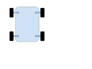
I needed to come up with some equations to use to steer a slow moving 4 wheeled robot shown in the following diagram. From this, you can see there are 4 wheel assemblies located at each corner of the robot’s platform. Each of the wheel assemblies has 2 independently controlled motors, one of which turns the wheel and a short “shaft” about a pivot point and the other motor propels the wheel itself. Each wheel assembly must be given a turning angle as well as a rotational speed. Given this setup, I started looking into how one might want to design a set of controls to steer it.
My first cut at this, is to define 4 different modes of steering:
- front wheel steering – In front wheel steering, only the front wheels are rotated about a fixed point while the rear wheels stay in a fixed position. This is how a typical automobile is steered.
- rear wheel steering – In rear wheel steering, we do the opposite. The front wheels are locked pointing straight ahead and the rear wheels are rotated about a fixed point.
- four wheel steering – In four wheel steering, the front and rear wheels are rotated around a single rotation point.
- crab steering – In crab steering, all wheels are rotated in the same direction having the same angle and the same rotational velocity. The equations for determining the angles and rotational velocities are trivial.
Because this robot is moving at slow speeds through out its course, I didn’t take into account issues such as slippage, cornering forces or other complications. With these simplifications, it turns out that if we are careful, we can treat the front wheel and rear wheel steering as special cases of the four wheel steering. Hence, we’ll derive the equations for the four wheel steering mode – that is, for turning 4 wheels about a single point of rotation as shown in the diagram below:
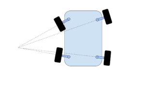
For this discussion, we’ll use a 2 dimensional rectangular coordinate with its origin midway between the two rear wheels. All the wheels will be rotating around the same rotation point as shown above. If you notice, the wheels need to be perpendicular to a radial line drawn from the rotation point at the coordinates (xr,yr) to their respective wheel posts.
Given that setup, let’s start deriving the equations that will ultimately give use the angles and velocities. To do this, we’ll first simplify this by assuming that the vehicle has just 2 wheels, i.e. that it is a bicycle.
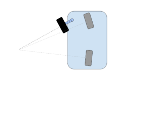
We’ll derive the angles and velocities for those two wheels and then we’ll calculate what the angles and velocities should be at each of four locations. In this diagram, you’ll see that the we’ve introduced 2 virtual wheels, a front and a rear shown in gray.

This vehicle has 4 independently steerable wheels. There is a wheel post around which a short shaft extends and can turn. At the other end of this shaft is the actual wheel.
We’ll use a rectangular coordinate system with the origin halfway between the 2 rear wheel posts. The positive x axis will point to the right rear wheel post. The positive y axis will point to the front of the vehicle.
We’re assuming the following:
- \( D \) := distance between front wheel and rear wheel posts.
- \( W \) := distance between the 2 front wheels.
- \( S \) := length of the shaft.
- \( \gamma_{lfp} \) := the angle our actual front left tire makes with the y axis. Note \(\gamma_{rfp}, \gamma_{rbp}, \gamma_{lbp}\) are the angles that the right front, right back and left back tires make with the y axis.
- \( \beta \) := the angle our imaginary front center tire makes with the y axis
- \( \alpha \) := the angle our imaginary rear center tire makes with the y axis
- \( (0,0) \) := the mid point between the 2 rear wheel posts
- \( (x_r, y_r) \) := the point of rotation.
- \( (x_{lfp}, y_{lfp}) \) := the location of the left front wheel post that the left front wheel assembly pivots about.
- \( r_{cf} \) := distance between the rotation point and the center front
- \( r_{cb} \) := distance between the rotation point and the center rear point. We’ll place the origin there.
- \( r_{lfp} \) := distance between the rotation point and the left front wheel post.
- \( r_{lfw} \) := distance between the rotation point and the middle of the left front wheel itself.
- \( \omega_{lfw} \) := the angular velocity of our actual left front tire. Note \(\omega_{rfw}, \omega_{rbw}, \omega_{lbw}\) are the angular velocities of the right front, right back and left back tires.
- \( v \) := The desired speed of the vehicle.
Derivation
We’ll assume that we are given \( \alpha \) and \( \beta \) since these will be supplied by our steering interface. A positive angle will cause the wheel to turn right and a negative one will turn it left. In our final equations, we’ll set these angles according to the steering mode as follows:
| Four wheel | in this mode, we set \( \beta = -\alpha\) |
| Front | \( \alpha \) is set while \( \beta = 0 \) |
| Rear | \( \beta \) is set while \( \alpha = 0 \) |
| Crab mode | in this mode, we set \( \beta = \alpha \) |
The easiest coordinate to determine other than the origin, is the location of the left front wheel post. This post sets at \( (-\frac{W}{2}, D) \). We can use the Sine law together with the trignometric identity \( sin(\frac{\pi}{2} – \theta)=cos(\theta)\) to determine the radial \( r_{cf} \) from \( (x_r, y_r)\) to the imaginary front center wheel. Similarly for \(r_{cb}\). This yields:
- \( r_{cf} = D \frac{cos \alpha}{sin( \alpha – \beta )}\)
- \( r_{cb} = D \frac{cos \beta}{sin( \alpha – \beta )}\)
We can also calculate \( x_r, y_r \) quite easily once we know \( r_{cb} \)
- \( x_r = -r_{cb} cos \alpha = -r_{cf} cos \beta \)
- \( y_r = r_{cb} sin \alpha \)
Finally after calculating \( x_r \) and \( y_r \), we can get \( r_{lfp} \) and \( \gamma_{lfp} \).
- \( r_{lfp} = \sqrt{ (x_r + \frac{W}{2})^2 + (D – y_r)^2 } \)
- \( \gamma_{lfp} = tan^{-1}(\frac{D-y_r}{x_r + \frac{W}{2}}) = sin^{-1}( \frac{D – y_r}{ r_{lfp} } ) \)
- \( r_{lfw} = r_{lfp} – S \)
Now we can also use the \( tan^{-1} \) to calculate the remaining angles \( \gamma_{rfp}, \gamma_{rbp}, \gamma_{lbp} \) as:
- \( \gamma_{rfp} = tan^{-1}( \frac{D-y_r}{x_r – \frac{W}{2}} ) \)
- \( \gamma_{rbp} = tan^{-1}( \frac{-y_r}{x_r – \frac{W}{2}} ) \)
- \( \gamma_{lbp} = tan^{-1}( \frac{-y_r}{x_r + \frac{W}{2}} ) \)
So we now have the turning angles for our wheels.
Speed
Next we need to determine the speed at which the right wheel should be traveling around its circle. We’re given the desired speed of the vehicle as \( v \). Using this, we can calculate how fast our imaginary front center wheel must revolve. We know that \( 1 revolution = 2 \pi radius_{cf} \) distance. So:
That’s the angular velocity of the imaginary center front wheel, but how do we get the angular velocities of the actual wheels? We note that all the wheels need to traverse the same arc angle around their respective circles during the turn. E.g. if we were to spin around 360o degrees, we’d expect all the wheels to travel around their circle’s circumference and finish at the same instant. The distance that they’d travel is proportional to the length of their radial. Let’s say that we need to make a 13o arc denoted by \(\theta\) about the point of rotation. Then the right front wheel will need to travel a distance \(r_{rfw} \theta \) while the left rear wheel will need to travel \( r_{lrw} \theta \) distance.
So if our desired rotation is \( \omega_{cf} \) around the front center point, we have:
- \( \omega_{rfw} = \omega_{cf} \frac{r_{rfw}}{r_{cf}} \)
- \( \omega_{rbw} = \omega_{cf} \frac{r_{rbw}}{r_{cf}} \)
- \( \omega_{lfw} = \omega_{cf} \frac{r_{lfw}}{r_{cf}} \)
- \( \omega_{lbw} = \omega_{cf} \frac{r_{lbw}}{r_{cf}} \)
Recap
Here are the full equations:
- \( r_{cf} = D \frac{cos \alpha}{sin( \alpha – \beta )}\) Where
- \( r_{cb} = D \frac{cos \beta}{sin( \alpha – \beta )}\)
- \( x_r = -r_{cb} cos \alpha = -r_{cf} cos \beta \)
- \( y_r = r_{cb} sin \alpha \)
- \( r_{lfp} = \sqrt{ (x_r + \frac{W}{2})^2 + (D – y_r)^2 } \)
- \( r_{rfp} = \sqrt{ (x_r – \frac{W}{2})^2 + (D – y_r)^2 } \)
- \( r_{lbp} = \sqrt{ (x_r + \frac{W}{2})^2 + (y_r)^2 } \)
- \( r_{rbp} = \sqrt{ (x_r – \frac{W}{2})^2 + (y_r)^2 } \)
- \( r_{lfw} = r_{lfp} – S \)
- \( r_{rfw} = r_{rfp} + S \)
- \( r_{lbw} = r_{lbp} – S \)
- \( r_{rbw} = r_{rbp} + S \)
- \( \gamma_{lfp} = tan^{-1}( \frac{D-y_r}{x_r + \frac{W}{2}} ) \)
- \( \gamma_{rfp} = tan^{-1}(\frac{D-y_r}{x_r – \frac{W}{2}}) \)
- \( \gamma_{lbp} = tan^{-1}( \frac{-y_r}{x_r + \frac{W}{2}} ) \)
- \( \gamma_{rbp} = tan^{-1}( \frac{-y_r}{x_r – \frac{W}{2}} ) \)
- \( \omega_{rfw} = \omega_{cf} \frac{r_{rfw}}{r_{cf}} \)
- \( \omega_{rbw} = \omega_{cf} \frac{r_{rbw}}{r_{cf}} \)
- \( \omega_{lfw} = \omega_{cf} \frac{r_{lfw}}{r_{cf}} \)
- \( \omega_{lbw} = \omega_{cf} \frac{r_{lbw}}{r_{cf}} \)
NOTE, that the equations are undefined when \( \alpha = \beta \) because the rotation point is effectively infinity. You should set both front tires to have the same angle as \( \beta \) and the rear tires to have the same angle as \( \alpha \) when the delta \( \alpha – \beta \) is very small.
Here is a spreadsheet contains the equations FourWheelSteeringEquations